Looking at cardiac data processing, feature extraction, and analysis in Python
ECG
HRV
Physiology
Timerseries
Signal Processing
GX dataset
EMG
Math
Author
Nigel Gebodh
Published
February 10, 2025
Image by DALLE-3 and Nigel Gebodh.
Here we look at an overview of the Electrocardiogram (ECG), its history, and analyzing and extracting features from ECG data.
What exactly is an ECG and some brief history?
ECG and History
Cardiac data can mean a lot of things. Generally it refers to data from or relating to the heart or cardiovascular system. The term cardiac comes from the Greek word kardia, and roughly translating to heart.
Here we’ll focus on looking at the electrocardiogram or ECG (or German elektrokardiogram- EKG) which measures the electrical activity of the heart over time. This non-invasive measurement provides critical insights into heart rhythm, function, and overall cardiovascular/ mental health.
The term electrocardiogram roughly breaks into:
electro - electricity
cardio - heart
gram - writing
Brief History
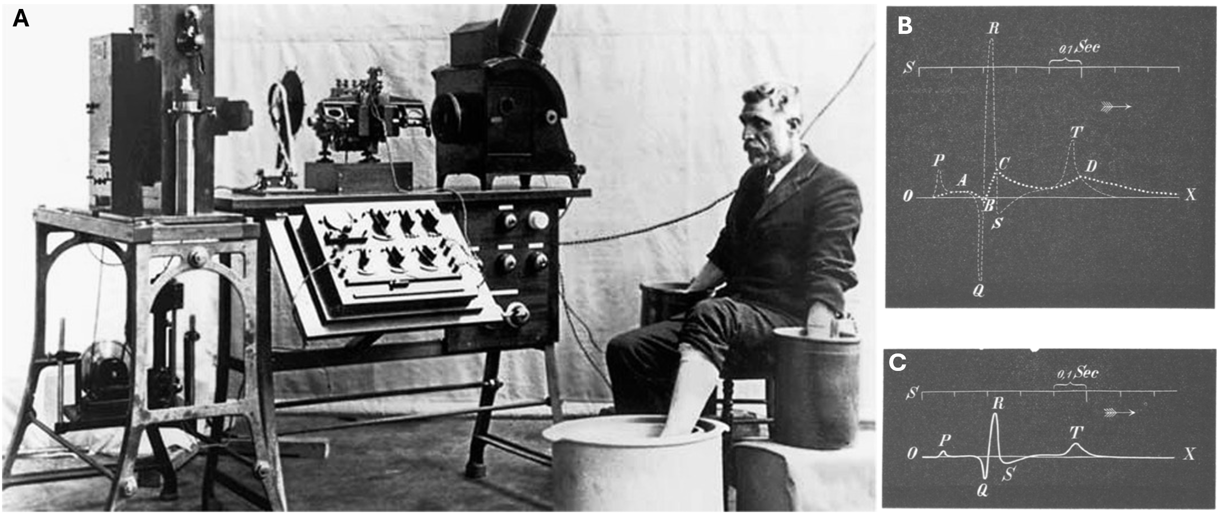
The typical ECG signal we know today is credited to work by Willem Einthoven between 1893-1895 (Einthoven, 1895). Einthoven, innovated on the work of Augustus Desire Waller (who introduced the term “electrocardiogram” ) and others by developing more sensitive and smaller detection instrumentation, which he called the string galvanometer(Einthoven, 1912).
With more sensitive equipment, Einthoven was able to discern more distinct cardiac peaks, which he labeled as the PQRST peaks. The naming convention is debated but it’s believed to be inspired by Einthoven’s study of work by Descartes (Hurst, 1998). Some of the earliest ECG machines were huge, required multiple operators, and patients had to have their arms and legs submerged in electrolyte (salty water) solutions. Einthoven was even approached by Charles Darwin’s son, Horace Darwin, to help sell and distribute the ECG machines (Burnett, 1985).
A. An early form of the ECG monitoring device. B-C. Einthoven’s correction and demarcation of points on the ECG waveform.
ECG Waveform
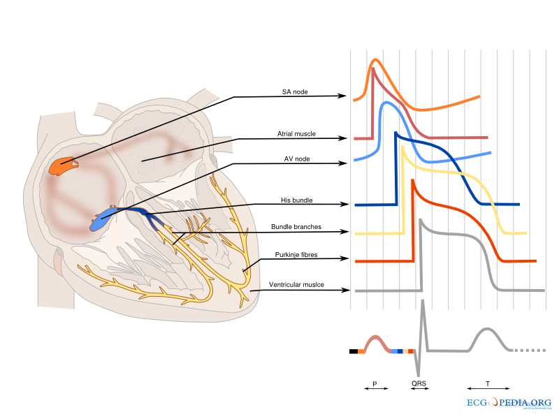
The ECG waveform reflects different phases of the heart’s contraction. Each of the PQRST points on the ECG waveform correspond to:
P wave - Atrial depolarization
QRS complex - Ventricular depolarization
T wave - Ventricular repolarization
The cardiac cycle and the origin of each part of the ECG waveform. Image source.
ECG in the Modern Era
Since its inception ECG acquisition has become digitized and miniaturized to the point where we can fit acquisition tools into a smart watch. Apple’s and other companies’ inclusion of such monitoring and diagnostic tools helped to democratize and increase access to cardiac health monitoring. Studies like the Apple Heart Study have demonstrated that wearable technology can accurately detect irregular heart rhythms, leading to earlier identification of conditions like atrial fibrillation and empowering users to take proactive steps in managing their heart health.
ECG in Context
ECG is a part of cardiac monitoring which is a broad term that encompasses a variety of methods for monitoring and assessing cardiac health. Taking a step back, we see ECG falls under EXG techniques, which is a term used to describe a group of non-invasive/minimally invasive methods that measure electrical activity in the body.
For example, some EXG techniques include:
Electromyography (EMG) - detection of electrical activity in muscles
Electroencephalography (EEG) - detection of electrical activity in the brain
Electrogastrography (EGG) - detection of electrical activity in the gut
Electrooculography (EOG) - detection of electrical activity in the eyes
Electroretinography (ERG) - detection of electrical activity in the retina
Note: While the heart is classified as a muscle, its muscle tissue differs significantly from skeletal muscle. The heart muscle cells, known as cardiomyocytes, and tissue have distinct anatomical features that set it apart from other muscles. Unlike skeletal muscle, which requires conscious control for contraction, cardiomyocytes possess the unique ability to contract and relax autonomously, without voluntary input. This fundamental difference is one of the key factors that distinguishes electrocardiography (ECG) from electromyography (EMG).
Other methods that monitor cardiac activity include:
Photoplethysmography - light based detection of blood volume changes in the skin
Phonocardiography - sound based detection of heart sounds
Ballistocardiography - detection of the force of the heart on the body
Impedance cardiography - detection of changes in the impedance of the chest
Let’s get Started
About the data
Details
The data that we’ll be working with here comes from one of my experiments looking at EEG, ECG, and vigilant behavior concurrently over time (Gebodh et al., 2021). We collected EEG and lead I ECG data over a 70-minute period while participants played a ball moving game and at times were stimulated with low intensity electrical stimulation (Check out my chapters on brain stimulation here(Moreno-Duarte et al., 2014) and here(Gebodh et al., 2019) ). We’ll focus on the first 20 minutes of data since its free from artifacts of electrical stimulation.
Snippet of the GX dataset. The data contains EEG, ECG, EOG, and behavioral data.
Processing Pipeline
Details
When working with signals it’s good practice to have a processing pipeline and adjust as needed. Here our processing pipeline will be to:
Import the data
Preprocess the data:
Remove baseline wandering. These low frequency drifts can happen because of sweat or changes in skin impedances. We can attenuate this activity by high-pass filtering the signal.
Remove high frequency noise. This can happen when muscles under the electrodes like the pectoral muscles are active causing the ECG waveform to become distorted and contaminated with EMG signals. We can attenuate this with low-pass filtering.
Downsample the signal. Since the signal is sampled at a high frequency (2k Hz) it contains more than enough samples to properly reconstruct the ECG signals so for faster processing we can downsample the signal to a lower frequency.
Extract ECG features
Downloading The Data
We’ll start off by downloading and importing the data.
The data are uploaded to the OpenNeuro database, which supports neuroscience data sharing, reproducibility, and analysis. Our data can be viewed here. The data are divided into different folders, each corresponding to a different participant (e.g. sub-01 corresponds to participant 1). Subfolders corresponding to different sessions (e.g. ses-02 corresponds to session 2).
To download the data, we can use curl, which is a command line tool for transferring data.
Long Explanation
For example in a Command Line Interface (CLI), like command prompt etc., we can run the following command to download the data to a specific folder:
curl<DATA URL> -o <OUTPUT FILE PATH &NAME>
The data files are broken into different files, each containing a different type of data. The main data files are:
.set and .fdt - contains the recorded timerseries data and metadata
.json - contains metadata for the experiment
.tsv - contains the events data (triggers) for the timeseries and EEG electrode locations
The URL for our data can be broken down as follows for participant 22, session 1:
Base URL: https://s3.amazonaws.com/openneuro.org/
Dataset ID: ds003670/
Participant folder: sub-022/
Session folder: ses-01/
Data type(all are the same): eeg/
File name: sub-022_ses-01_task-GXtESCTT_eeg.json
So, the full DATA URL for the file we want to download is:
Once the data is downloaded, we can import it using mne. From there we can extract segments to process and visualize.
Code
import mneimport numpy as npimport bokehtemp_folder ='./temp_data'file_in ='sub-001_ses-001_task-rest_eeg'ecg_electrodes =32# ECG electrode# Load the data# Set preload=False to use memory mapping (lazy loading)raw = mne.io.read_raw_eeglab(f'{temp_folder}{file_in}.set', preload=False)# Load the TSV file - contains events (remove `_eeg` from the end of the file name)events_df = pd.read_csv(f'{temp_folder}{file_in[:-3]}events.tsv', sep='\t')sfreq = raw.info['sfreq']# Data sampling frequency# Extract the ECG data for the first 10 secondsstart, stop =0, 30# in secondsdata, times = raw[ecg_electrodes, start * sfreq :stop * sfreq ]# Plot the ECG data with Bokehp = bokeh.plotting.figure(title="EEG Data", x_axis_label='Time (s)', y_axis_label='Amplitude')p.line(times, data[0])show(p)
Let’s look at a snippet of the data.
Loading BokehJS ...
What do we see?
If we look closely at the signal, we notice a few things:
Signal offset. On the y-axis the signal is offset from zero. This is because the signal is measured with respect to a reference point and there is a large potential difference between both the electrodes and the reference point.
Signal drift. We notice that the signal is drifting (it’s not constantly centered at ~-2.5 mV). We can see the drift line (Low-Freq Drift) in the plot. Drifting is a common problem in ECG signals (typically 0.05-1 Hz) and can be caused by a number of factors, including changes in the participant’s position, body temperature, or the electrode-skin interface.
Signal noise. We can see that the signal has some high frequency noise. This is highlighted in the plot (High-Freq Noise) and looks like sharp spikes (typically 20-1k Hz). In this case this was most likely caused by the movement of the participant’s arms, which results in detecting electrical signals from the underlying muscles (or an electromyographic -EMG signal).
Data Preprocessing
Filtering
We can attenuate (reduce) some of this unwanted activity in the ECG signal by filtering it. We’ll apply a high pass filter to remove the low frequency noise (drift, offset etc.) and a low pass filter to remove the high frequency noise (EMG noise etc.). It’s important to note that filtering can distort the signal and attenuate fiducial points on the ECG waveform so the bandlimits of the filters should be chosen carefully. Typically, most of the useful frequency content of an ECG waveform is between 0.5-40 Hz.
Here we’ll use the Butterworth filter (an IIR filter) to filter the ECG signal. The Butterworth filter has a maximally flat frequency response in the passband, meaning it results in minimal distortion to the signal. Other types of IIR filters include the Chebyshev filter, Bessel filter, and elliptic filter.
There are many other filtering techniques that can be used to remove noise from/clean ECG data (other than high/low/band pass filtering). These include (reviewed in Chatterjee et al. (2020) ):
Adaptive filtering
Wavelet filtering
Empirical mode decomposition
Singular spectrum analysis
Kalman filtering
Deep learning based filtering (e.g. autoencoders)
Code
# Import librariesfrom scipy import signal# Filtering# High pass filterdef high_pass_filter(data, fs, cutoff, order=4):#Design filter with Butterworth filter function b, a = signal.butter(order, cutoff/(fs/2), 'highpass')return signal.filtfilt(b, a, data)#Filter forward and backward# Low pass filterdef low_pass_filter(data, fs, cutoff, order=3):#Design filter with Butterworth filter function b, a = signal.butter(order, cutoff/(fs/2), 'lowpass')return signal.filtfilt(b, a, data)#Filter forward and backward# Apply filtersfiltered_hp = high_pass_filter(data, fs, 0.5)filtered_lp = low_pass_filter(data, fs, 25)
When we filter the signal, we get:
Time domain signals
Loading BokehJS ...
Frequency domain signals
What do we see?
After filtering we see that:
The voltage offset in the filtered signal is now ~0.
The low frequency drift in the signal is now gone. Its stable around 0 over time.
The majority of the high frequency noise is gone.
In the frequency domain we can see that the high frequency noise is attenuated more than that in the unfiltered signal (>20 Hz).
We can use the peak PSD in the frequency domain to roughly estimate the average heart rate from our ECG segment.
We can do more processing to clean the signal further, but this should be good enough to extract some useful features from the signal.
Downsampling
Downsampling is the process of reducing the sampling rate of a signal. This is done to reduce the amount of data that needs to be processed, and to make the signal easier to work with. For example, if we downsample our signal from 2000 Hz to 100 Hz, we are reducing the amount of data by a factor of 20 (2000 Hz/ 100 Hz = 20 reduction factor).
Generally, when downsampling follow the rules of the Nyquist–Shannon sampling theorem, which states that the sampling rate of a signal must be at least twice the highest frequency component of the signal of interest.
For example, if I recorded a signal that I know has a maximum frequency of 100 Hz, then I would need to sample the signal at least 200 Hz (100 Hz* 2 = 200 Hz). If I oversampled my signal, I could downsample it to about 200 Hz and still be able to reconstruct the original signal, any lower than that and I could lose information.
Code
import scipy.signal as signalfs =1000fs_down =100#Calculate the downsampling factordownsample_factor = fs // fs_down# 1000 // 100 = 10, so downsample by factor of 10#Downsample the signal data_ds = resample_poly(data, up=1, down=downsample_factor)
Below is an extreme example of downsampling, where we downsample from 2000 Hz to 150 Hz.
What do we see?
After downsampling (from 2000 Hz to 150 Hz) the signal we that:
There are much less samples in the downsampled signal
This can speed up the processing
The downsampled signal still retains the characteristics (PQRST) of the original signal
Data Feature Extraction
Now that we’ve cleaned the data, we can extract features from it.
One of the most common features used in ECG analysis is the heart rate, which can be extracted in a number of ways. The most common way is to use the R-peaks from the detected QRS complex.
Pan-Tompkins Algorithm
The Pan-Tompkins algorithm, developed in 1985 by Jiapu Pan and Willis J Tompkins(Pan & Tompkins, 1985) is one of the most common ways to extract the QRS-complex, get the R-peaks and then calculate the heart rate.
The algorithm can be broken down into the following steps:
Bandpass Filtering: Filter the signal between 5 and 15 Hz.
Low pass filter below 15 Hz
High pass filter above 5 Hz
Differentiation: Perform a first order derivative.
Take the difference between the current sample and the previous sample.
Squaring: Square each sample of the signal.
Moving Window Integration: Integrate over signal in a moving window.
Thresholding: Scan the original ECG signal for peaks above a certain threshold using the integrated signal.
Signal here refers to the outcome from each previous step.
For example, we can code the Pan-Tompkins algorithm in Python and run it on our dataset to detect QRS complexes and the R-peaks. From there we can use the R-peaks to calculate the heart rate, heart rate variability, and other interesting metrics.
Code
#Simplified Pan-Tompkins algorithmclass PanTompkinsQRS:""" Implementation of Pan-Tompkins QRS detection algorithm """def__init__(self, sampling_rate=250):self.sampling_rate = sampling_rate# Bandpass filter (5-15 Hz)def bandpass_filter(self, signal):""" Bandpass filter (5-15 Hz) """ nyquist_freq =self.sampling_rate /2 low =5/ nyquist_freq high =15/ nyquist_freq b, a = butter(1, [low, high], btype='band') ecg_filt = filtfilt(b, a, signal)return ecg_filt # Differentiationdef differentiation(self, signal):""" Differentiation """ ecg_diff = np.diff(signal)#Pad with a number at the beginning pad_loc =0#Index to add pad pad_val = ecg_diff[0] ecg_diff = np.insert(ecg_diff , pad_loc, pad_val)return ecg_diff # Squaringdef squaring(self, signal):""" Squaring """ ecg_sqr = signal **2return ecg_sqr# Moving Window Integration/ Moving averagedef moving_average(self, signal, window_size=0.150#In sec ):""" Moving average Parameters: - window_size: in sec """ window_size =int(window_size *self.sampling_rate) kernel = np.ones(window_size) / window_size ecg_mov_avg = np.convolve(signal, kernel, mode='same')return ecg_mov_avg#Find Peaks within the signaldef find_R_peaks(self, processed_signal, raw_signal):""" Find R-peaks using thresholding. - `processed_signal`: The moving average output (used for thresholding) - `raw_signal`: The original filtered ECG signal (to find the true R-wave) """ peak_distance =int(0.250*self.sampling_rate) # ~250ms between heartbeats peak_prominence =0.5* np.max(processed_signal) # Dynamic threshold# 1. Detect approximate peaks in processed signal peaks, _ = find_peaks(processed_signal, distance=peak_distance, prominence=peak_prominence)# 2. Search for the true R-peak in the raw ECG signal r_peaks = [] search_window =int(0.050*self.sampling_rate) # Search ±50ms around each detected peakfor peak in peaks: search_region = raw_signal[max(0, peak - search_window):min(len(raw_signal), peak + search_window)] true_r_peak = np.argmax(search_region) + (peak - search_window) # Shift index to raw signal r_peaks.append(true_r_peak)return np.array(r_peaks)# QRS detectiondef qrs_detection(self, signal):""" QRS detection """ signal = signal - np.mean(signal) ecg_filt =self.bandpass_filter(signal) ecg_diff =self.differentiation(ecg_filt) ecg_sqr =self.squaring(ecg_diff) ecg_mov_avg =self.moving_average(ecg_sqr) ecg_r_peaks =self.find_R_peaks(ecg_mov_avg, signal)# Return the results as a dictionaryreturn {"signal": signal,"ecg_filt": ecg_filt,"ecg_diff": ecg_diff,"ecg_sqr": ecg_sqr,"ecg_mov_avg": ecg_mov_avg,"ecg_r_peaks": ecg_r_peaks }
What do we see?
From the plot, we can see that:
The Pan-Tompkins algorithm is able to accurately detect the R-peaks in the ECG signal.
HR & HRV Extraction
There are several updated algorithms for automatic extraction of R-peaks and the QRS complex from the ECG signal. In Python the NeuroKit2 package contains a function for the Pan-Tompkins algorithm along with other updated algorithms.
Here we’ll use the NeuroKit2 package to extract the R-peaks and QRS complex from the ECG signal and run some basic analysis to get HR and HRV.
HR
Code
#====================================================# Data Extraction#----------------------------------------------------# Get some dataraw, events_df = load_data(file_in, './temp_data/')sfreq = fs = raw.info['sfreq']# Data sampling frequency# Extract the EEG datastart, stop =5, 15# in secondsdata, times = raw[32, start * sfreq :stop * sfreq ]data = data[0]*1e3fs = fs_down =250#Downsampledata = downsample_to_frequency(data , sfreq, fs_down)data = signal.detrend(data)times = np.linspace(start,stop, num=len(data))#____________________________________________________# Process ecgecg_cleaned = nk.ecg_clean(data, sampling_rate=fs)signals_out_pre, info_pre = nk.ecg_process(ecg_cleaned , sampling_rate=fs)nk.ecg_plot(signals_out_pre, info_pre)fig = plt.gcf()# Set the figure sizefig.set_size_inches(12, 10) # Adjust the size as needed# Show the plotplt.show()
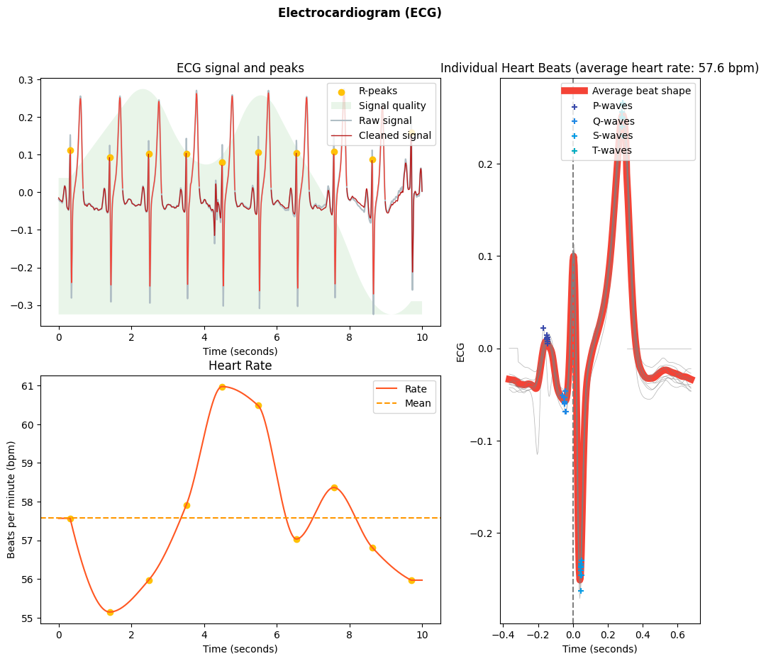
What do we see?
From the plot above, we can see that:
The built-in algorithm was able to detect the majority of the R-peaks.
We can calculate the instantaneous heart rate between two consecutive R-peaks.
We can aggregate all the ECG waveforms to get a sense of the overall ECG signal.
HRV
Code
#====================================================# Data Extraction#----------------------------------------------------# Get some dataraw, events_df = load_data(file_in, './temp_data/')sfreq = fs = raw.info['sfreq']# Data sampling frequency# Extract the EEG datastart, stop =0, 60*10# in secondsdata, times = raw[32, start * sfreq :stop * sfreq ]data = data[0]*1e3fs = fs_down =250#Downsampledata = downsample_to_frequency(data , sfreq, fs_down)data = signal.detrend(data)times = np.linspace(start,stop, num=len(data))#____________________________________________________# Clean signal and Find peaksecg_cleaned = nk.ecg_clean(data, sampling_rate=fs)peaks, info = nk.ecg_peaks(ecg_cleaned, sampling_rate=fs, correct_artifacts=True)# Compute HRV indiceshrv_indices = nk.hrv(peaks, sampling_rate=fs, show=True)fig = plt.gcf()# Set the figure sizefig.set_size_inches(12, 10) # Adjust the size as needed # Show the plotplt.show()
What do we see?
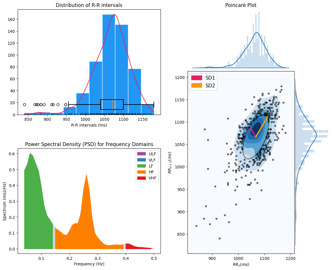
Here we look at a 10-minute segment of ECG data. From the plot above, we can see that:
We can aggregate all the RR intervals to get a sense of the heart rate variability (HRV) over the whole segment.
More or less variation in the RR intervals indicate the balance between the sympathetic and parasympathetic nervous systems.
The balance between the sympathetic and parasympathetic nervous systems can further be examined by looking at the balance between the high frequency(HF-orange) and low frequency (LF-green) components of spectrum of the RR intervals.
The Poincare plot shows the relationship between consecutive RR intervals. Within the plot we see that the long-term variability (SD2; slower fluctuations) is higher than the short-term variability (SD1; faster fluctuations).
HR & HRV Data Summary
For the HR and HRV data extraction, we obtained cardiac metrics from the time domain and frequency domain.
Time Domain Metrics
Mean and Median RR Interval
Mean and Median RR Interval
This is the average time between all of the RR intervals (\(\overline{RR}\)) in the given data segment. We calculate it as:
where \(RR_i\) is the \(i^{th}\) RR interval, \(\overline{RR}\) is the mean RR interval, and \(n\) is the number of RR intervals.
For our data:
SDNN: 48.706 ms
Root Mean Square of Successive Differences (RMSSD)
Root Mean Square of Successive Differences (RMSSD)
This metric provides information about the variability in the time between consecutive RR intervals. We calculate it as: \[
\text{RMSSD} = \sqrt{\frac{1}{n-1} \sum_{i=1}^{n-1} (RR_{i+1} - RR_i)^2}
\] where \(RR_i\) is the \(i^{th}\) RR interval, and \(n\) is the number of RR intervals.
For our data:
RMSSD: 44.845 ms
Percentage of RR Interval Differences > 50 ms (pNN50)
Percentage of RR Interval Differences > 50 ms (pNN50)
This metric quantifies the percentage of consecutive RR intervals that differ by more than 50 ms. We calculate it as: \[
\text{NN50} = \sum_{i=1}^{n-1} \mathbb{1}_{|RR_i - RR_{i+1}| > 50}
\]
where \(NN50\) is the number of consecutive RR intervals that differ by more than 50 ms.
For our data:
PNN50: 24.242 %
Frequency Domain Metrics
Total Power (TP)
Total Power (TP)
This metric represents the total power in the frequency domain. We calculate it as: \[
\text{TP} = \int_{0}^{0.5} P(f) \, df
\] where \(P(f)\) is the power spectral density(PSD) of the RR intervals.
For our data:
TP: 0.053 \(ms^2\)
Low Frequency Power (LF)
Low Frequency Power (LF)
This metric represents the power in the low frequency range (0.04-0.15 Hz). We calculate it as:
where \(P(f)\) is the power spectral density(PSD) of the RR intervals.
For our data:
HF: 0.018 \(ms^2\)
Low Frequency/High Frequency Ratio (LF/HF)
Low Frequency/High Frequency Ratio (LF/HF)
This metric represents the ratio of high frequency power to low frequency power. We calculate it as: \[
\text{LF/HF Ratio} = \frac{LF_{power}}{HF_{power}}
\]
For our data:
LF/HF: 1.066
Outcomes summarized:
Time Domain Metrics:
Mean RR Interval
Median RR Interval
SDNN
RMSSD
pNN50
1066.86
1072
48.7062
44.8448
24.2424
Frequency Domain Metrics:
Total Power
Low Freq Power
High Freq Power
Low Freq/High Freq Ratio
0.0527402
0.0196355
0.0184252
1.06569
Take Away
The electrocardiogram (ECG) has become a gold standard for monitoring cardiac and overall health, providing valuable insights beyond traditional diagnostics. We explored how ECG data can be processed to extract meaningful physiological markers such as heart rate (HR) and heart rate variability (HRV), which are key indicators used to detect arrhythmias, autonomic nervous system activity, and mental health states.
With advancements in machine learning and wearable technology, ECG analysis is evolving beyond conventional applications. AI-driven algorithms can enhance early disease detection, personalized health monitoring, and real-time stress and wellness assessment. The integration of ECG data with machine learning not only refines diagnostics but also opens new frontiers in preventative healthcare, digital therapeutics, and remote patient monitoring. This paves the way for continuous, intelligent ECG monitoring; empowering individuals to proactively manage their heart health and overall well-being.
Cite as
@misc{Gebodh2025FromHeartBeatstoAlgorithmsWithECGData,
title = {From Heart Beats to Algorithms With ECG Data},
author = {Nigel Gebodh},
year = {2025},
url = {https://ngebodh.github.io/projects/Short_dive_posts/ECG_analysis/ECG_proc.html},
note = {Published: February 10, 2025}
}
Chatterjee, S., Thakur, R. S., Yadav, R. N., Gupta, L., & Raghuvanshi, D. K. (2020). Review of noise removal techniques in ECG signals. IET Signal Processing, 14(9), 569–590. https://doi.org/https://doi.org/10.1049/iet-spr.2020.0104
Einthoven, W. (1895). Ueber die form des menschlichen electrocardiogramms. Archiv Für Die Gesamte Physiologie Des Menschen Und Der Tiere, 60(3), 101–123. https://doi.org/10.1007/BF01662582
Gebodh, N., Esmaeilpour, Z., Adair, D., Schestattsky, P., Fregni, F., & Bikson, M. (2019). Transcranial direct current stimulation among technologies for low-intensity transcranial electrical stimulation: Classification, history, and terminology. In H. Knotkova, M. A. Nitsche, M. Bikson, & A. J. Woods (Eds.), Practical guide to transcranial direct current stimulation: Principles, procedures and applications (pp. 3–43). Springer International Publishing. https://doi.org/10.1007/978-3-319-95948-1_1
Gebodh, N., Esmaeilpour, Z., Datta, A., & Bikson, M. (2021). Dataset of concurrent EEG, ECG, and behavior with multiple doses of transcranial electrical stimulation. Scientific Data, 8(1), 274. https://doi.org/10.1038/s41597-021-01046-y
Hurst, J. W. (1998). Naming of the waves in the ECG, with a brief account of their genesis. Circulation, 98(18), 1937–1942. https://doi.org/10.1161/01.CIR.98.18.1937
Moreno-Duarte, I., Gebodh, N., Schestatsky, P., Guleyupoglu, B., Reato, D., Bikson, M., & Fregni, F. (2014). Chapter 2 - transcranial electrical stimulation: Transcranial direct current stimulation (tDCS), transcranial alternating current stimulation (tACS), transcranial pulsed current stimulation (tPCS), and transcranial random noise stimulation (tRNS). In R. Cohen Kadosh (Ed.), The stimulated brain (pp. 35–59). Academic Press. https://doi.org/https://doi.org/10.1016/B978-0-12-404704-4.00002-8
Pan, J., & Tompkins, W. J. (1985). A real-time QRS detection algorithm. IEEE Transactions on Biomedical Engineering, BME-32(3), 230–236. https://doi.org/10.1109/TBME.1985.325532