Nigel Gebodh
  • Home
  • Publications
  • Talks & Media
  • Projects
  • Connect
    • Google Scholar
    • LinkedIn
    • Twitter(X)
    • GitHub
    • YouTube
    • BlueSky
    • nigel.gebodh@gmail.com

On this page

  • Project Overview
  • Import Libraries
  • Load the Data
  • Data Exploration
  • Data Preprocessing
  • Build the Model
  • Compile the Model
  • Calculating the number of parameters for each layer
    • Layer 1
    • Layer 2
    • Layer 3
  • Train the model
    • Training Accuracy Visualization
    • Plot the accuracy of the training model
    • Training vs. Validation Accuracy
    • Training vs. Validation: Accuracy and Loss
    • Model Evaluation on Test Data
  • Archived

Digit Recognition with MLP from Scratch

Using a MLP to classify digits

Deep Learning
ML
Computer Vision
Image Recognition
TensorFlow
Keras
Author

Nigel Gebodh

Published

January 1, 2022


Cover_image

Digit Recognition. Photo by Nick Hillier on Unsplash


Project Overview

This notebook demonstrates the development of a neural network classifier using Keras to recognize handwritten digits from the MNIST dataset. The MNIST dataset is a widely used benchmark in machine learning, consisting of 70,000 grayscale images of handwritten digits (0-9). We will preprocess the images, build a multi-layer perceptron (MLP) model, train it, and evaluate its performance.

The process involves:

  1. Data Loading: Importing the MNIST dataset.
  2. Data Exploration: Understanding the structure and format of the image data.
  3. Data Preprocessing: Reshaping, normalizing, and one-hot encoding the data.
  4. Model Building: Constructing a neural network architecture.
  5. Model Compilation: Configuring the learning process.
  6. Model Training: Fitting the model to the training data.
  7. Model Evaluation: Assessing the model’s accuracy on the test data.
  8. Visualization: Plotting training and validation accuracy and loss.

Import Libraries

We begin by importing the necessary libraries:

  • NumPy: For numerical operations.
  • Keras (TensorFlow): For building and training the neural network.
  • Matplotlib: For data visualization.
from keras.datasets import mnist
from keras.preprocessing.image import load_img, array_to_img
from keras.utils.np_utils import to_categorical
from keras.models import Sequential
from keras.layers import Dense

import numpy as np
import matplotlib.pyplot as plt
%matplotlib inline
Using TensorFlow backend.

Load the Data

We load the MNIST dataset, which is conveniently provided by Keras.

(X_train, y_train), (X_test, y_test) = mnist.load_data()
Downloading data from https://s3.amazonaws.com/img-datasets/mnist.npz
11493376/11490434 [==============================] - 1s 0us/step

Data Exploration

Let’s examine the shape of the loaded data.

print(type(X_train))
print(X_train.shape)
print(y_train.shape) #60k is the answers
print(X_test.shape)  #10K entries
print(y_test.shape)
<class 'numpy.ndarray'>
(60000, 28, 28)
(60000,)
(10000, 28, 28)
(10000,)

This shows that we have 60,000 training images and 10,000 test images, each of size 28x28 pixels.

Let’s visualize a sample image and its corresponding label.

#Lets look at the data to see what it looks like
print(X_train[0].shape) #Look at the size of the 1st entry

#Plot it to see what it looks like

plt.imshow(X_train[0])

#Print the answer
print("The answer is {}".format(y_train[0]))
(28, 28)
The answer is 5

Data Preprocessing

We need to preprocess the image data before feeding it into the neural network.

  • Reshape: Flatten the 28x28 images into 784-dimensional vectors.
  • Normalize: Scale the pixel values to the range [0, 1].
  • One-Hot Encode: Convert the labels into a categorical format.
image_height, image_width =28, 28
#Lets reshape each image to be a single vector rather than a matrix

#Have to flatten to plug into neural net

X_train  =X_train.reshape(60000,image_height*image_width)

X_test   =X_test.reshape(10000,image_height*image_width)
print(X_train.shape) #28X28 =784
print(X_test.shape)
(60000, 784)
(10000, 784)
#Check to see if image is between 0-255
print(min(X_train[0]), max(X_train[0])) #it is! so we need to normalize

#We will convert data to float (insead of int) to scale the data betwn 0-1 (not 0-255)

X_train = X_train.astype('float32') #Convert to float
X_test  = X_test.astype('float32') #Convert to float
0 255
#Normalize the data
X_train /= 255.0
X_test  /= 255.0
print(min(X_train[0]), max(X_train[0])) #Normalized
0.0 1.0
# We want the output to be in one of 9 bins to rep each of the 0-9 numbers
#In order to do this we can convert the answers to a categorical value
#We do this using the 'to_categorical' method

y_train =to_categorical(y_train, 10)
y_test  =to_categorical(y_test, 10)
print(y_train.shape)
print(y_test.shape)
(60000, 10)
(10000, 10)
print(y_test[0])
plt.imshow(X_test[0].reshape(image_height, image_width))
[0. 0. 0. 0. 0. 0. 0. 1. 0. 0.]

Build the Model

We construct a sequential neural network model with three dense layers.

#Assign the model type
model = Sequential()
WARNING: Logging before flag parsing goes to stderr.
W0820 07:17:37.393794 140395328268160 deprecation_wrapper.py:119] From /usr/local/lib/python3.6/dist-packages/keras/backend/tensorflow_backend.py:74: The name tf.get_default_graph is deprecated. Please use tf.compat.v1.get_default_graph instead.
#Add layers to the model

model.add(Dense(512, activation='relu',input_shape=(784,)))
model.add(Dense(512, activation='relu'))
model.add(Dense(10, activation='softmax'))
W0820 07:17:37.444703 140395328268160 deprecation_wrapper.py:119] From /usr/local/lib/python3.6/dist-packages/keras/backend/tensorflow_backend.py:517: The name tf.placeholder is deprecated. Please use tf.compat.v1.placeholder instead.

W0820 07:17:37.461894 140395328268160 deprecation_wrapper.py:119] From /usr/local/lib/python3.6/dist-packages/keras/backend/tensorflow_backend.py:4138: The name tf.random_uniform is deprecated. Please use tf.random.uniform instead.

Compile the Model

We compile the model with the Adam optimizer, categorical cross-entropy loss, and accuracy metric.

model.compile(optimizer='adam', loss='categorical_crossentropy', metrics=['accuracy'])
W0820 07:17:37.521929 140395328268160 deprecation_wrapper.py:119] From /usr/local/lib/python3.6/dist-packages/keras/optimizers.py:790: The name tf.train.Optimizer is deprecated. Please use tf.compat.v1.train.Optimizer instead.

W0820 07:17:37.561933 140395328268160 deprecation_wrapper.py:119] From /usr/local/lib/python3.6/dist-packages/keras/backend/tensorflow_backend.py:3295: The name tf.log is deprecated. Please use tf.math.log instead.
model.summary()
_________________________________________________________________
Layer (type)                 Output Shape              Param #   
=================================================================
dense_1 (Dense)              (None, 512)               401920    
_________________________________________________________________
dense_2 (Dense)              (None, 512)               262656    
_________________________________________________________________
dense_3 (Dense)              (None, 10)                5130      
=================================================================
Total params: 669,706
Trainable params: 669,706
Non-trainable params: 0
_________________________________________________________________

Calculating the number of parameters for each layer

Layer 1

  • After flattening each image we get:
    • 28 X 28=784
  • We then pass the 784 into 512 nodes in the model plus a bias layer 512 (zeros)
  • This gives:
    • 784(pixels) X 512(neurons) X 512(bias)=401920

Layer 2

  • We have 512 (output from previous), going into another 512 nodes (in new layer), plus another 512
  • This gives:
    • 512 (input) X 512 (this layer) X 512 =262656

Layer 3

  • We have 512 (incoming from last layer), going into 10 nodes (in this layer), 10 bias units
  • This gives:
    • 512 (last layer) X 10 (nodes in this layer) + 10 (bias) =5130

Train the model

Now we can train our model. To do this we have to pass: * Training data * Number of epochs (the number of times that model passes through the training data) * Validation data (testing data)

history =model.fit(X_train, y_train, epochs =20, validation_data=(X_test, y_test))
W0820 07:17:37.736055 140395328268160 deprecation.py:323] From /usr/local/lib/python3.6/dist-packages/tensorflow/python/ops/math_grad.py:1250: add_dispatch_support.<locals>.wrapper (from tensorflow.python.ops.array_ops) is deprecated and will be removed in a future version.
Instructions for updating:
Use tf.where in 2.0, which has the same broadcast rule as np.where
W0820 07:17:37.796303 140395328268160 deprecation_wrapper.py:119] From /usr/local/lib/python3.6/dist-packages/keras/backend/tensorflow_backend.py:986: The name tf.assign_add is deprecated. Please use tf.compat.v1.assign_add instead.
Train on 60000 samples, validate on 10000 samples
Epoch 1/20
60000/60000 [==============================] - 24s 394us/step - loss: 0.1828 - acc: 0.9440 - val_loss: 0.0929 - val_acc: 0.9705
Epoch 2/20
60000/60000 [==============================] - 23s 386us/step - loss: 0.0808 - acc: 0.9757 - val_loss: 0.0827 - val_acc: 0.9743
Epoch 3/20
60000/60000 [==============================] - 23s 389us/step - loss: 0.0565 - acc: 0.9828 - val_loss: 0.0695 - val_acc: 0.9786
Epoch 4/20
60000/60000 [==============================] - 23s 381us/step - loss: 0.0429 - acc: 0.9864 - val_loss: 0.0832 - val_acc: 0.9774
Epoch 5/20
60000/60000 [==============================] - 23s 386us/step - loss: 0.0353 - acc: 0.9887 - val_loss: 0.0921 - val_acc: 0.9745
Epoch 6/20
60000/60000 [==============================] - 23s 387us/step - loss: 0.0287 - acc: 0.9910 - val_loss: 0.0819 - val_acc: 0.9782
Epoch 7/20
60000/60000 [==============================] - 23s 387us/step - loss: 0.0272 - acc: 0.9914 - val_loss: 0.0807 - val_acc: 0.9802
Epoch 8/20
60000/60000 [==============================] - 24s 395us/step - loss: 0.0237 - acc: 0.9924 - val_loss: 0.1136 - val_acc: 0.9771
Epoch 9/20
60000/60000 [==============================] - 23s 390us/step - loss: 0.0201 - acc: 0.9938 - val_loss: 0.1083 - val_acc: 0.9800
Epoch 10/20
60000/60000 [==============================] - 23s 381us/step - loss: 0.0202 - acc: 0.9939 - val_loss: 0.1016 - val_acc: 0.9798
Epoch 11/20
60000/60000 [==============================] - 23s 390us/step - loss: 0.0170 - acc: 0.9951 - val_loss: 0.1167 - val_acc: 0.9783
Epoch 12/20
60000/60000 [==============================] - 23s 387us/step - loss: 0.0175 - acc: 0.9948 - val_loss: 0.1026 - val_acc: 0.9805
Epoch 13/20
60000/60000 [==============================] - 23s 381us/step - loss: 0.0179 - acc: 0.9950 - val_loss: 0.1039 - val_acc: 0.9811
Epoch 14/20
60000/60000 [==============================] - 23s 377us/step - loss: 0.0155 - acc: 0.9956 - val_loss: 0.1173 - val_acc: 0.9809
Epoch 15/20
60000/60000 [==============================] - 22s 374us/step - loss: 0.0179 - acc: 0.9947 - val_loss: 0.1135 - val_acc: 0.9801
Epoch 16/20
60000/60000 [==============================] - 25s 415us/step - loss: 0.0126 - acc: 0.9965 - val_loss: 0.1391 - val_acc: 0.9792
Epoch 17/20
60000/60000 [==============================] - 24s 397us/step - loss: 0.0151 - acc: 0.9964 - val_loss: 0.1211 - val_acc: 0.9819
Epoch 18/20
60000/60000 [==============================] - 24s 400us/step - loss: 0.0159 - acc: 0.9962 - val_loss: 0.1208 - val_acc: 0.9800
Epoch 19/20
60000/60000 [==============================] - 24s 403us/step - loss: 0.0166 - acc: 0.9960 - val_loss: 0.1309 - val_acc: 0.9808
Epoch 20/20
60000/60000 [==============================] - 24s 397us/step - loss: 0.0133 - acc: 0.9965 - val_loss: 0.1310 - val_acc: 0.9813

Training Accuracy Visualization

To understand how well our model learned during the training phase, we can visualize the training accuracy over each epoch. The history object, returned by the model.fit() method, stores the training metrics. We’ll plot the ‘acc’ key from this dictionary, which represents the training accuracy, against the epoch number.

This graph will show us how the model’s accuracy improved as it was exposed to more training data. Ideally, we should see a steady increase in accuracy over epochs.

Plot the accuracy of the training model

#Look at the attributes in the history object to find the accuracy
history.__dict__
{'epoch': [0,
  1,
  2,
  3,
  4,
  5,
  6,
  7,
  8,
  9,
  10,
  11,
  12,
  13,
  14,
  15,
  16,
  17,
  18,
  19],
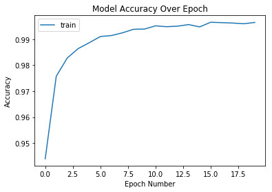
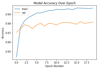
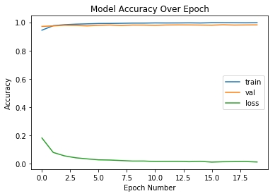
 'history': {'acc': [0.9439666666666666,
   0.9757333333333333,
   0.9827833333333333,
   0.9864166666666667,
   0.9886666666666667,
   0.9910333333333333,
   0.9914,
   0.99245,
   0.9938166666666667,
   0.9939,
   0.99515,
   0.9948,
   0.9950166666666667,
   0.9956333333333334,
   0.9947333333333334,
   0.9965166666666667,
   0.9963833333333333,
   0.9962166666666666,
   0.99595,
   0.99645],
  'loss': [0.1827596818920225,
   0.08079896697839722,
   0.05645396511411139,
   0.04291815567353721,
   0.03526910000597515,
   0.02873079521368248,
   0.02715607473684601,
   0.023650182965393438,
   0.020055528101623546,
   0.02019607128013062,
   0.016955279541049723,
   0.017472221146037314,
   0.017864977817751575,
   0.015457480643335983,
   0.017869793417473495,
   0.012631182595215281,
   0.015135916414613901,
   0.015882995463786898,
   0.016569432756344288,
   0.013335457366452594],
  'val_acc': [0.9705,
   0.9743,
   0.9786,
   0.9774,
   0.9745,
   0.9782,
   0.9802,
   0.9771,
   0.98,
   0.9798,
   0.9783,
   0.9805,
   0.9811,
   0.9809,
   0.9801,
   0.9792,
   0.9819,
   0.98,
   0.9808,
   0.9813],
  'val_loss': [0.09286645495379343,
   0.08266143489209934,
   0.069480553943431,
   0.08320518101718044,
   0.09206652115154429,
   0.08190068501315655,
   0.08067529291427782,
   0.11358439496830543,
   0.10833151409866154,
   0.10160923933375093,
   0.11671308373045626,
   0.10255490619101375,
   0.10387474813488247,
   0.11728941089477675,
   0.11347036018394005,
   0.13906407877868832,
   0.12108565404413693,
   0.120797497302599,
   0.1309188434239974,
   0.13095201672244552]},
 'model': <keras.engine.sequential.Sequential at 0x7fb0320f3400>,
 'params': {'batch_size': 32,
  'do_validation': True,
  'epochs': 20,
  'metrics': ['loss', 'acc', 'val_loss', 'val_acc'],
  'samples': 60000,
  'steps': None,
  'verbose': 1},
 'validation_data': [array([[0., 0., 0., ..., 0., 0., 0.],
         [0., 0., 0., ..., 0., 0., 0.],
         [0., 0., 0., ..., 0., 0., 0.],
         ...,
         [0., 0., 0., ..., 0., 0., 0.],
         [0., 0., 0., ..., 0., 0., 0.],
         [0., 0., 0., ..., 0., 0., 0.]], dtype=float32),
  array([[0., 0., 0., ..., 1., 0., 0.],
         [0., 0., 1., ..., 0., 0., 0.],
         [0., 1., 0., ..., 0., 0., 0.],
         ...,
         [0., 0., 0., ..., 0., 0., 0.],
         [0., 0., 0., ..., 0., 0., 0.],
         [0., 0., 0., ..., 0., 0., 0.]], dtype=float32),
  array([1., 1., 1., ..., 1., 1., 1.], dtype=float32)]}
#Plot the accuracy
plt.plot(history.history['acc'],label='train')
plt.xlabel('Epoch Number')
plt.ylabel('Accuracy')
plt.title('Model Accuracy Over Epoch')
plt.legend()

Training vs. Validation Accuracy

To assess if our model is generalizing well to unseen data, we’ll compare the training accuracy with the validation accuracy. The validation accuracy is calculated on the test dataset during training, providing insights into how the model performs on data it hasn’t been explicitly trained on.

By plotting both training and validation accuracies, we can identify potential overfitting. If the training accuracy is significantly higher than the validation accuracy, it might indicate that the model is memorizing the training data rather than learning general patterns.

#Plot the accuracy of training data and validation data
plt.plot(history.history['acc'],label='train')
plt.plot(history.history['val_acc'],label='val')
plt.xlabel('Epoch Number')
plt.ylabel('Accuracy')
plt.title('Model Accuracy Over Epoch')
plt.legend()

Training vs. Validation: Accuracy and Loss

In addition to accuracy, the loss function provides valuable information about the model’s performance. The loss represents the error between the model’s predictions and the actual labels.

#Plot the accuracy of training data and validation data AND loss
plt.plot(history.history['acc'],label='train')
plt.plot(history.history['val_acc'],label='val')
plt.plot(history.history['loss'],label='loss')
plt.xlabel('Epoch Number')
plt.ylabel('Accuracy')
plt.title('Model Accuracy Over Epoch')
plt.legend()
# plt.yscale('log')

Model Evaluation on Test Data

After training our model, we need to evaluate its performance on unseen data to assess its generalization ability.

score=model.evaluate(X_test, y_test)
10000/10000 [==============================] - 1s 84us/step
#We get score as a list
#The second item in score gives us the accuracy of or model
score
[0.13095201672244552, 0.9813]

Archived

Project Archive Note:

This project is archived.
Please note that library and framework versions may be outdated.
Last updated:

  • April 2025

© Nigel Gebodh, Made on Earth by a Human